Large area geophysical metal detector survey

[99thpercentile]

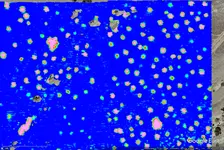
Here are some example results from almost 20 years ago utilizing the Geonics EM63 time domain electromagnetic induction (TDEM) metal detector. At the time the EM63 was the most advanced metal detector in the world for detecting and discriminating unexploded ordnance (UXO). The large coil on the bottom is the transmitter coil and the three smaller coils in the middle are the receiver coils. The receiver coils made a differential measurement between the coils over 27 time gates (recordings spaced in time after the transmitter turns off). The system operates at approximately 10 Hz, so at a normal walking speed of 1 m/s we would have one measurement every 10 cm. The system actually operates at closer to 100 Hz, but averages the data down to 10 Hz to increase the signal to noise ratio. After several years of testing, it was determined that to maximize the functionality of these types of systems that we needed not only data at multiple times on the decay curve but that we also needed better geometry to improve our understanding of the target. This system would be considered a digital geophysical mapping (DGM) instrument while the newest generation of instruments fall into the advanced geophysical classification (AGC) category. We processed the data in Geosoft Oasis Montaj software for basic data cleanup and presenation. We then used the data in the University of British Columbia's (UBC) UXOLab software to perform advanced target detection.

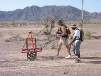
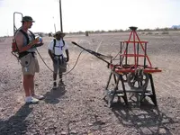
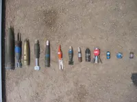
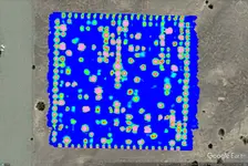
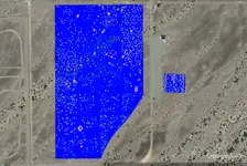
The data was collected at 0.5 m line spacing over the entire site over a period of about a month. The mapped data shows the open field area (the very large area) as well as the calibration site next to it. For the calibration site we knew where all of the targets were, what they were, and their exact depth and orientation. For the open field area, the goal was to detect all of the targets, determine what they were, and their exact location and orientation. I also have a zoomed in picture of the calibration area as well as a zoomed in picture of the open field area. The pictures show myself and my colleague Eric pushing the EM63 with a Trimble RTK GPS receiver attached to it as well as the EM63 up on plastic sawhorses for a calibration measurement. I also included a picture of most of the types of UXO buried at this site.

Let me know if you have any questions about what I have shown here.

 

Amazon Forum Fav 👍

DR.ÖTEK Metal Detector, Waterproof Gold Detector, Pinpoint & Terrain Modes, Professional Metal Detector - Grab it through Amazon!

[plum702]

its interesting that it is only in the hz range

 

[cyzak]

I just wanna say thank you for this information you’re sharing. It is providing so much information about how these systems work.

 

[99thpercentile]

its interesting that it is only in the hz range

Sorry if there was some confusion on operating frequency.

All electromagnetic induction instruments operate in the high Hz to mid-kHz range (~100 Hz to ~50 kHz) in terms of the waveform.

The Geonics EM61-MK2 is a bipolar time domain instrument. That means that it turns on, stays on, then turns off as an approximate square wave. That square wave repeats at approximately 70 Hz. The 10 Hz that I mentioned is a function of the stacking (i.e. how many successive measurement are averaged to reduce noise). The newest version of the instrument outputs data at 18 Hz.

The frequency content or bandwidth of the measurement is really a function of how quickly the instrument can turn off each transmit pulse. Instruments that can turn off very quickly have high frequency content. This is a function of the inductance of the coil and the instrument electronics. This turn on/off is balanced against how many turns the coil has as a way increase the effective area of the coil. Larger effective area coils, combined with higher current, can generate larger signals and detect deeper targets. Unfortunately, if the effective area is too large you can't turn off quickly and may not detect small shallow targets.

Everything in instrument design is a series of compromises.

 

[99thpercentile]

I just wanna say thank you for this information you’re sharing. It is providing so much information about how these systems work.

You are welcome.

I do this for several reasons.

Treasure hunting is fun so by educating others I sometimes get to go on paid treasure hunting jobs. This is obviously self serving, but it has worked for me in the past. I like to get paid to do what I went to school for many years to do, but occasionally I even do jobs at cost or below cost if they sound really cool. I will pretty much never volunteer to show up at a site for free and bring my $50K to $100K at my own expense.

Most treasure hunters don't have geophysics degrees so don't have the practical and theoretical background in doing these types of surveys every day as a job. There are a lot of unscrupulous equipment manufacturers out there who try to sell widgets to treasure hunters that are blatant rip offs. The treasure hunters who are terrified of the prices of real geophysical instruments really hope that these unscrupulous vendors aren't going to essentially steal from them, but they are. If you can see what the real instruments do, then you will know what to expect and hopefully avoid some of these vendors. If a $5K to $10K instrument could do the same thing as my $30K to $100K instrument, we would be buying those instead and using them. Are real geophysical instruments more expensive than they should be, absoluting, but this is just a supply/demand problem. Most of the near surface geophysics equipment manufacturers just don't sell enough units to lower costs.

I gladly answer questions about how geophysicists go about solving these problems.

 

[plum702]

I have been reading your post since I puchased my gpr about 15 years ago which was an expensive mistake for Las Vegas ground is very rocky and the rocks look like plastic pipes the only thing that tells us it’s a pipe is we can see the trench. I do pipe locating and there is great application for locators for prospecting

 

[pepperj]

The last photo shows all the target spots.
Are they all ordinances?

 

[ConceptualizedNetherlandr]

Was that a salted hunt to test the capabilities?

 

[99thpercentile]

The last photo shows all the target spots.
Are they all ordinances?

Many of the targets are UXO, but many are not.

This is one of the two Standardized UXO Test Sites. The goal is to evaluate how well different sensors work. There are two small grids called the calibration grid and the blind grid. The large are is called the open field site.

On the calibration grid you are provided a map with the exact location, depth, and orientation of each target as well as exactly what it is.

For the blind grid you are given the location of each target but no other information. The goal is to determine what it is, the depth, Nd the orientation.

For the open field site you are just provided the boundaries. The goal is to locate all of the buried targets, determine their depth, determine their orientation, classify them as UXO or non-UXO and if they are UXO identify what model they are.